Value iteration on `FrozenLake-v0` (Python)

In this example, we use the value iteration algorithm to train an agent on the FrozenLake-v0 environment. In PyCubeAI there is a tabular implementation of the algorithm implemented in the ValueIteration class.

Imports needed to run the example.

import gym
import numpy as np
import matplotlib.pyplot as plt

from src.algorithms.dp.value_iteration import ValueIteration, DPAlgoConfig
from src.algorithms.rl_serial_agent_trainer import RLSerialTrainerConfig, RLSerialAgentTrainer
from src.policies.uniform_policy import UniformPolicy
from src.policies.max_action_equal_probability_stochastic_policy_adaptor import MaxActionEqualProbabilityAdaptorPolicy
from src.worlds.world_helpers import n_states, n_actions

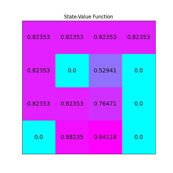
Next we implement a helper function for plotting the value function

def plot_values(v: np.array) -> None:

    # reshape value function
    V_sq = np.reshape(v, (4, 4))

    # plot the state-value function
    fig = plt.figure(figsize=(6, 6))
    ax = fig.add_subplot(111)
    im = ax.imshow(V_sq, cmap='cool')
    for (j, i), label in np.ndenumerate(V_sq):
        ax.text(i, j, np.round(label, 5), ha='center', va='center', fontsize=14)
    plt.tick_params(bottom=False, left=False, labelbottom=False, labelleft=False)
    plt.title('State-Value Function')
    plt.show()

Finally, we put everything together. The driver starts with a UniformPolicy instance which we initalize with the number of states and actions of the environment.

if __name__ == '__main__':

        ENV_NAME = "FrozenLake-v0"
        GAMMA = 1.0

        env = gym.make(ENV_NAME)
        policy_init = UniformPolicy(n_actions=n_actions(env),
                                   n_states=n_states(env), init_val=None)

        policy_adaptor = MaxActionEqualProbabilityAdaptorPolicy()

        agent_config = DPAlgoConfig(gamma=GAMMA, tolerance=1.0e-10, policy=policy_init)

        agent = ValueIteration(agent_config, policy_adaptor)

        trainer_config = RLSerialTrainerConfig(n_episodes=1000,
                                               tolerance=1.0e-10, output_msg_frequency=100)

        trainer = RLSerialAgentTrainer(config=trainer_config, agent=agent)
        ctrl_res = trainer.train(env)

        print(f"Converged {ctrl_res.converged}")
        print(f"Number of iterations {ctrl_res.n_itrs}")
        print(f"Residual {ctrl_res.residual}")

        print("\nOptimal Policy (LEFT = 0, DOWN = 1, RIGHT = 2, UP = 3):")
        print(agent.policy.policy, "\n")

        plot_values(agent.v)

Running the driver code above produces the following output

INFO: Episode 0 of 1000, (0.1% done)
INFO Done. Execution time 0.0010964580005747848 secs
INFO Done. Execution time 0.0009977879999496508 secs
INFO Done. Execution time 0.00101123800050118 secs
INFO Done. Execution time 0.000928472999476071 secs
INFO Done. Execution time 0.0008954209997682483 secs
INFO Done. Execution time 0.0008632760000182316 secs
INFO Done. Execution time 0.0008822680001685512 secs
INFO Done. Execution time 0.0009741799995026668 secs
...
INFO Done. Execution time 0.6396229520005363 secs
Converged True
Number of iterations 591
Residual 1e-12

Optimal Policy (LEFT = 0, DOWN = 1, RIGHT = 2, UP = 3):
[[1.   0.   0.   0.  ]
 [0.   0.   0.   1.  ]
 [0.   0.   0.   1.  ]
 [0.   0.   0.   1.  ]
 [1.   0.   0.   0.  ]
 [0.25 0.25 0.25 0.25]
 [0.5  0.   0.5  0.  ]
 [0.25 0.25 0.25 0.25]
 [0.   0.   0.   1.  ]
 [0.   1.   0.   0.  ]
 [1.   0.   0.   0.  ]
 [0.25 0.25 0.25 0.25]
 [0.25 0.25 0.25 0.25]
 [0.   0.   1.   0.  ]
 [0.   1.   0.   0.  ]
 [0.25 0.25 0.25 0.25]]

The image below shown the value function produced

Value iteration on FrozenLake-v0 (Python)

Value iteration on `FrozenLake-v0` (Python)